ComputerVision

Final ProjectPage
A semi-empirical billiards and pool tracker

Lampros Kourtis - Marios Philiastides - Constantinos Stratelos

1. Proposal

We are proposing a tracking algorithm for the game of billiards (pool). Our system will track multiple objects (the pool balls) at the same time and it will solve the correspondence problem, namely it will assign each ball a number corresponding to its actual game number. Our goal is to make decisions about the status of the game, i.e. whether a specific ball is still on the table, or whether a ball was pocketed etc.

The tentative outline of our algorithm for a minimum functionality is as follows:

  • A sequence of color images will be the input.
  • The images are converted to grayscale.
  • An edge detection algorithm converts each frame to a binary image containing the principal edges detected in the grayscale image.
  • Now the algorithm branches to two different steps:
    • We detect the table boundaries and estimate the projective geometry of the scene.
    • Use the table boundaries to run the ball detection part
  • Use the estimated geometry to infer the 'true' positions of the balls on the pool table.


2. The motivation

We are great pool players but we've always had some minor conflicts between us when a shot was not very clear. So we tought that it would be a nice idea to make use of the algorithms we learned in CS223B and also use our profound knowledge of billiards to improve this - not so much acknowledged - sport.


3. The real motivation

We just had to do a final project!!!


4. Data

We gathered data from a real 8 - ball pool game at the recreation area at Rains Houses graduate residences at Stanford University.

Here is a sample:


5. Algorithms

Here is the control flow block diagram of our algorithm:

The control flow of our algorithm

Let's take a step - by - step look at our algorithm:

5. 1. Edge detection

We used Matlab's built in function for edge detection and chose the Canny algorithm. Choosing the right low and high thresholds was not an easy task. For now these are hard - coded so that they give the optimal results for the view points of our data and for the lighting of the scenes. In a more sophisiticated implementation they could be determined automatically.

5. 2. Detecting the table boundaries and geometry.

The key algorithm behind our project was the Hough transform.

We implemented two different versions of the algorithm. One for fitting lines on the scene and one for fitting circles.

But how does Hough transform work?

5. 2. 1 Hough transform in a nutshell.

The main idea behind this brilliant algorithm is a transformation of image features, namely edges, to a space where it is more obvious where straight lines are formed, as well as other parametric curves, depending on the programmer's choice. The following image shows the Hough transform for lines.

For each pixel on an edge, the transform computes its distance from the center of the image and the angle that the position vector forms. If we then plot all these (distance, angle) pairs we get the right image. All the points on the same line form curves that pass through the same point.

Now it is obvious which points belong to the same line in the original image.

Hough transform for straight lines


5. 2. 2 Computing bounding boxes, geometry and perspective.

5. 2. 2. 1 Bounding box.

In order to compute the bounding box of the pool table we ran our Hough lines algorithm on the edges of the scene. This revealed all the straight lines. First we computed the line with the minimum distance from the center of the table and erased the lines with the same slope as this one. By doing this we were able to recursively compute the 4 lines that form the bounding box of the table.

5. 2. 2. 2 Geometry.

The four corners of the table were computed by looking at all possible intersections of the 4 bounding lines and then determining the one with the 4th smallest distance from the centroid (the mean in both directions) of those intersections. We by throwing away the points with distances bigger than this we were left with the 4 corners of the table.

5. 2. 2. 3 Inverse perspective matrix computation.

We have measured the dimensions of our table so that we know the true coordinates of our table. By combining the estimated corners on the image plane with the true ones we were able to compute the inverse perspective transformation matrix.

The inverse perspective mapping.

What we did was to try to find a 3 X 3 matrix that would map each point on the image plane onto the world (or table) plane.

The most difficult task here was to make sure that both the image plane and the table plane had the same center. In order to make sure that this is the case we translated the table plane and then when the mapping was done we translated back.

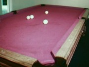
5. 3. Detecting the balls.

Having detected the table corners we ran our implementation of Hough transform for circles on the region of interest defined by the bounding box.

For each ball a triplet was computed, namely the center coordinates and the radius .

We used Hough transform again parametrized for circles.

Hough transform for circles.

Hough transform in general is a voting algorithm. In the case of circles for each pixel on an edge and for each radius in a given range of interest a circle is drawn. The pixels where most circles go through accumulate more votes and come up as maxima in the accumulator array. For a specific sensitivity of the algorithm one can apply a threshold to the accumulator and discover the first n strongest center pixels.

For our case here is a 3D surf plot of one of our accumulators.

5. 4. Table bird's eye view.

Constructing the table as seen from above was an easy task once the inverse perspective transform matrix was available. We took the centers of the balls in homogenous coordinates, mapped them to the table plane and rehomogenized the transformed centers by dividing by their 3rd component (w).

For the visualization of this part we used a trick. We constructed two images. One depicting the table from above and one for a ball. (The color of the ball is not relevant - we are only interested in the geometry of the scene). Then for each of the transformed centers we glued (by changing the pixels) the ball image on the table image.


6. Implementation

We used Matlab 6.0 for the implemenation of our algorithms.

6. 1 Source code.

  • main.m - The script that runs everything
  • findLines.m - A function that takes an image and returns the 4 lines that form the bounding box pf the pool table.
  • getPerspective.m - A function that given 4 pairs of points on the (u, v) plane (the image plane) and the (x, y) plane (the world or table plane) returns a 3 X 3 matrix that performs the inverse perspective mapping.
  • getBallCenters.m - Function that computes the ball centers and paints everything (lines and circles) on the original image.
  • houghCircles.m - The core of our algorithm. Hough transform for circles.


7. Results - conclusions

7. 1 Results of our algorithm.

Here is a picture showing the results from the several steps of our algorithm.

Our algorithm in action.

Let's go through them one by one:

a. The original RGB image. b. The accumulator for the lines. c. The lines found are drwan on the grayscale version of the original image. d. The accumulator for the circles confined in the bounding box of the table. e. The accumulator is smoothed with a gaussian kernel and then a threshold is applied, in order to identify the most significant accumulating positions in Hough space. f. The ball centers and radii have been computed and drawn on the original RGB image.

And here are the videos we made:


And combined:

and another one

7. 2 Outstanding problems.

  • We used a web - cam to shoot our videos. Due to the poor quality of the camera the nonlinear distortion of the images was a big problem. The scene colors were saturated. Most of the balls appeared white which did not allow us to implement one of our original ideas, which was to do color segmentation in order to identify the balls by name and assign their respective numbers.
  • If one of the lines detected by the Hough transform passes through the table and very close to its center then our scheme for detecting the 4 lines that form the bounding box breaks.
  • Sometimes the computed radii are not quite correct, but for our goals this didn't introduce serious problems since we were only interested in the position of the balls.

7. 3 Conclusions.

We tried to make a tracker for the game of pool and billiards. We researched the numerous computer vision algorithms for the ones that would be most suitable for our purposes. At the same time we wanted to make a program based on our ideas and not just implement already exhausted areas.

In our search for good ideas we discovered Hough transform and realized that it would serve our project in the best way. It turns out that Hough was an invaluable tool but also posed several challenges and problems. The core of the algorithm worked remarkably well but that wasn't enough. We had to come up with solutions to original problems. One of them was detecting the 4 relevant lines out of the many lines that Hough could reveal on the original image.

The other thread of our algorithm had to do with the inverse mapping from the image plane to the (x, y) plane of the pool table. We went through the literature and discovered that the problem was relativily difficult to handle. We had to invent a way to make sure that the mapping would work for any geometry. In order to do so we thought of a way to make sure that the reference points on the (x, y) plane had the same centroid as the corners of the table on the image plane. That was required because we had no information about the translation of the center of the image with respect to the center of the real table.


8. References

[1]. A Computational Approach to Edge Detection
John Canny, IEEE Trans. on PAMI, 679-698, 1986.

[2]. Good Features to Track
J. Shi & C. Tomasi, Proc. of IEEE Conf. on Computer Vision and Pattern Recognition, 1994

[3]. Shape and Motion for Image Streams under Orthography: a Factorization Method
C. Tomasi & T. Kanade, TR-92-1270, Cornell University, March 1992.

[4]. The Condensation Tracking Algorithm
Michael Isard and Andrew Blake. (See website for publications and demos)

[5] Introductory Techniques for 3-D Computer Vision
Emanuele Trucco, Alessandro Verri, Prentice Hall, 1998


9. Links

10. Disclaimer

The authors of this page wish to make known that the tracker introduced here will not improve your pool and billiard skills. Please do not assume that this is a real life tool. It is just our class final project demo.

Copyright © 2002 Lampros Kourtis - Marios Philiastides - Constantinos Stratelos

Last Update: March 15, 2002 12:39 PM


Data | Algorithms | Implementation | Results | References | Code
CS223B